基于向量加权平均值的高效优化算法(Matlab代码实现)
📝个人主页:研学社的博客
💥💥💞💞欢迎来到本博客❤️❤️💥💥
🏆博主优势:🌞🌞🌞博客内容尽量做到思维缜密,逻辑清晰,为了方便读者。
⛳️座右铭:行百里者,半于九十。
目录
💥1 概述
📚2 运行结果
🎉3 参考文献
🌈4 Matlab代码实现
💥1 概述
本文介绍了一种名为weIghted meaN oF vectOrs(INFO)的创新优化算法的分析和原理,以优化不同的问题。INFO是一种改进的权重均值方法,其中加权均值思想用于固体结构,并使用三个核心过程更新向量的位置:更新规则,向量组合和局部搜索。更新规则阶段基于基于平均值的定律和收敛加速来生成新的向量。向量组合阶段创建获得的向量与更新规则的组合,以实现有希望的解决方案。改进了信息更新规则和载体组合步骤,提高了勘探开发能力。此外,局部搜索阶段有助于该算法摆脱低精度解决方案,并提高开发和收敛性。在48个数学测试函数和5个约束工程测试用例中评估了INFO的性能。根据文献,结果表明,INFO在勘探和开发方面优于其他基本和高级方法。在工程问题的情况下,结果表明,INFO可以收敛到全局最优解的0.99%。因此,INFO算法是优化问题中优化设计的一种很有前途的工具,这源于该算法在优化约束工况方面具有相当的效率。
📚2 运行结果
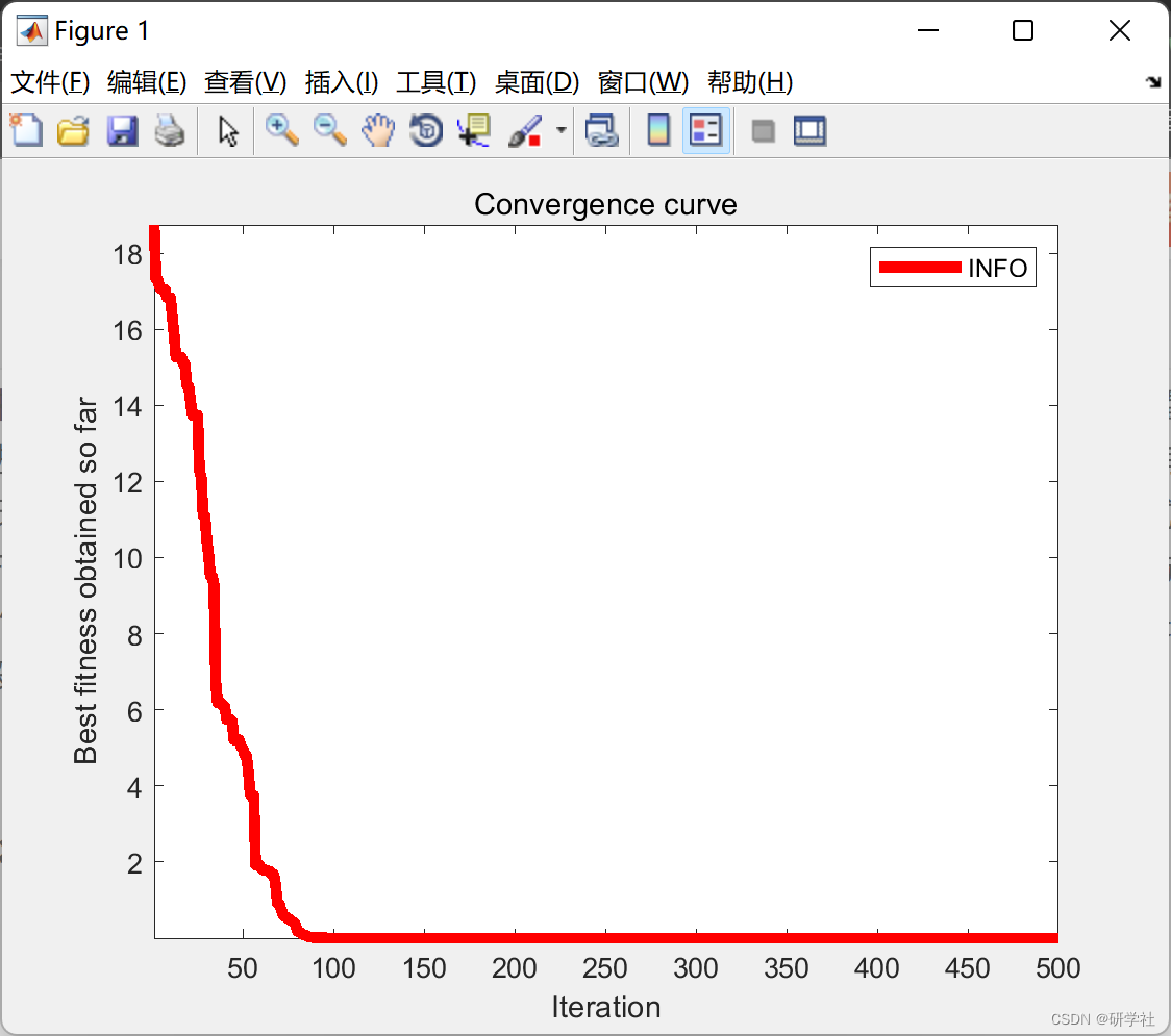
部分代码:
function [Best_Cost,Best_X,Convergence_curve]=INFO(nP,MaxIt,lb,ub,dim,fobj)
%% Initialization
Cost=zeros(nP,1);
M=zeros(nP,1);
X=initialization(nP,dim,ub,lb);
for i=1:nP
Cost(i) = fobj(X(i,:));
M(i)=Cost(i);
end
[~, ind]=sort(Cost);
Best_X = X(ind(1),:);
Best_Cost = Cost(ind(1));
Worst_Cost = Cost(ind(end));
Worst_X = X(ind(end),:);
I=randi([2 5]);
Better_X=X(ind(I),:);
Better_Cost=Cost(ind(I));
%% Main Loop of INFO
for it=1:MaxIt
alpha=2*exp(-4*(it/MaxIt)); % Eqs. (5.1) & % Eq. (9.1)
M_Best=Best_Cost;
M_Better=Better_Cost;
M_Worst=Worst_Cost;
for i=1:nP
% Updating rule stage
del=2*rand*alpha-alpha; % Eq. (5)
sigm=2*rand*alpha-alpha; % Eq. (9)
% Select three random solution
A1=randperm(nP);
A1(A1==i)=[];
a=A1(1);b=A1(2);c=A1(3);
e=1e-25;
epsi=e*rand;
omg = max([M(a) M(b) M(c)]);
MM = [(M(a)-M(b)) (M(a)-M(c)) (M(b)-M(c))];
W(1) = cos(MM(1)+pi)*exp(-abs(MM(1)/omg)); % Eq. (4.2)
W(2) = cos(MM(2)+pi)*exp(-abs(MM(2)/omg)); % Eq. (4.3)
W(3)= cos(MM(3)+pi)*exp(-abs(MM(3)/omg)); % Eq. (4.4)
Wt = sum(W);
WM1 = del.*(W(1).*(X(a,:)-X(b,:))+W(2).*(X(a,:)-X(c,:))+ ... % Eq. (4.1)
W(3).*(X(b,:)-X(c,:)))/(Wt+1)+epsi;
omg = max([M_Best M_Better M_Worst]);
MM = [(M_Best-M_Better) (M_Best-M_Better) (M_Better-M_Worst)];
W(1) = cos(MM(1)+pi)*exp(-abs(MM(1)/omg)); % Eq. (4.7)
W(2) = cos(MM(2)+pi)*exp(-abs(MM(2)/omg)); % Eq. (4.8)
W(3) = cos(MM(3)+pi)*exp(-abs(MM(3)/omg)); % Eq. (4.9)
Wt = sum(W);
WM2 = del.*(W(1).*(Best_X-Better_X)+W(2).*(Best_X-Worst_X)+ ... % Eq. (4.6)
W(3).*(Better_X-Worst_X))/(Wt+1)+epsi;
% Determine MeanRule
r = unifrnd(0.1,0.5);
MeanRule = r.*WM1+(1-r).*WM2; % Eq. (4)
if rand<0.5
z1 = X(i,:)+sigm.*(rand.*MeanRule)+randn.*(Best_X-X(a,:))/(M_Best-M(a)+1);
z2 = Best_X+sigm.*(rand.*MeanRule)+randn.*(X(a,:)-X(b,:))/(M(a)-M(b)+1);
else % Eq. (8)
z1 = X(a,:)+sigm.*(rand.*MeanRule)+randn.*(X(b,:)-X(c,:))/(M(b)-M(c)+1);
z2 = Better_X+sigm.*(rand.*MeanRule)+randn.*(X(a,:)-X(b,:))/(M(a)-M(b)+1);
end
% Vector combining stage
u=zeros(1,dim);
for j=1:dim
mu = 0.05*randn;
if rand <0.5
if rand<0.5
u(j) = z1(j) + mu*abs(z1(j)-z2(j)); % Eq. (10.1)
else
u(j) = z2(j) + mu*abs(z1(j)-z2(j)); % Eq. (10.2)
end
else
u(j) = X(i,j); % Eq. (10.3)
end
end
% Local search stage
if rand<0.5
L=rand<0.5;v1=(1-L)*2*(rand)+L;v2=rand.*L+(1-L); % Eqs. (11.5) & % Eq. (11.6)
Xavg=(X(a,:)+X(b,:)+X(c,:))/3; % Eq. (11.4)
phi=rand;
Xrnd = phi.*(Xavg)+(1-phi)*(phi.*Better_X+(1-phi).*Best_X); % Eq. (11.3)
Randn = L.*randn(1,dim)+(1-L).*randn;
if rand<0.5
u = Best_X + Randn.*(MeanRule+randn.*(Best_X-X(a,:))); % Eq. (11.1)
else
u = Xrnd + Randn.*(MeanRule+randn.*(v1*Best_X-v2*Xrnd)); % Eq. (11.2)
end
end
% Check if new solution go outside the search space and bring them back
New_X= BC(u,lb,ub);
New_Cost = fobj(New_X);
if New_Cost
Cost(i)=New_Cost;
M(i)=Cost(i);
if Cost(i)
Best_Cost = Cost(i);
end
end
end
% Determine the worst solution
[~, ind]=sort(Cost);
Worst_X=X(ind(end),:);
Worst_Cost=Cost(ind(end));
% Determine the better solution
I=randi([2 5]);
Better_X=X(ind(I),:);
Better_Cost=Cost(ind(I));
% Update Convergence_curve
Convergence_curve(it)=Best_Cost;
% Show Iteration Information
disp(['Iteration ' num2str(it) ',: Best Cost = ' num2str(Best_Cost)]);
end
end
function X = BC(X,lb,ub)
Flag4ub=X>ub;
Flag4lb=X
end
🎉3 参考文献
部分理论来源于网络,如有侵权请联系删除。
[1]Ahmadianfar, Iman, et al. “INFO: An Efficient Optimization Algorithm Based on Weighted Mean of Vectors.” Expert Systems with Applications, Elsevier BV, Jan. 2022, p. 116516, doi:10.1016/j.eswa.2022.116516.